Matthias enjoys bringing people together in the age-old process of sharing our collective knowledge.

With over 10 years of field experience, Matthias has studied the soundscapes of Hawai’i, monitored bird migration on the Colorado plateau in Oregon, and surveyed wildfire recovery in the Great Plains.
Returning home to Vermont, Matthias began working with the Forest Ecosystem Monitoring Cooperative with a focus on bringing it all together, looking at natural systems as a whole. A recent graduate from UVM Field Naturalist Program, Matthias is interested in work that makes data meaningful.
Highlighted work
Sugaring and Wildlife
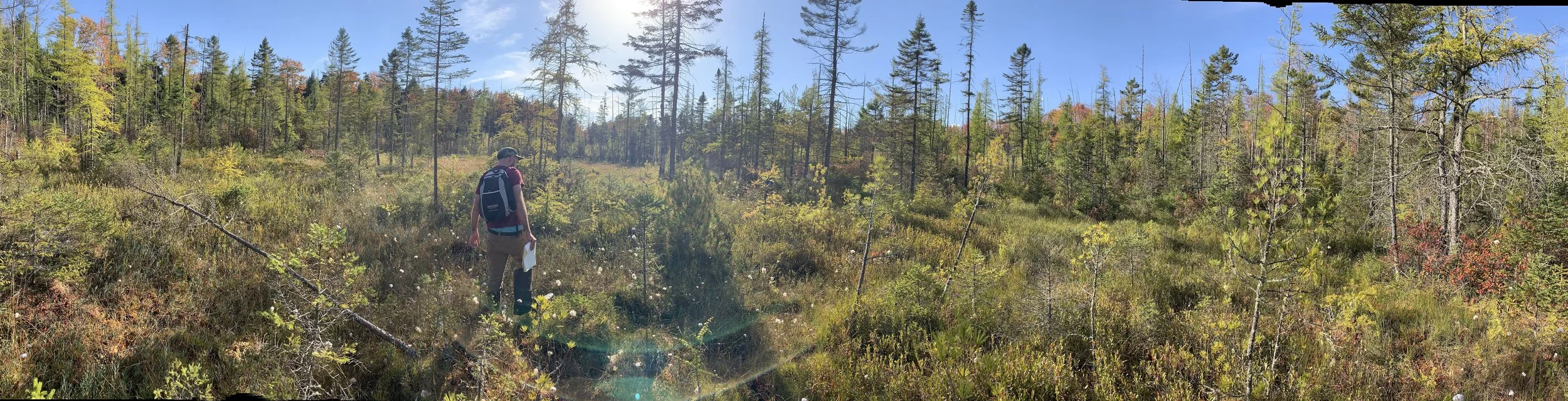
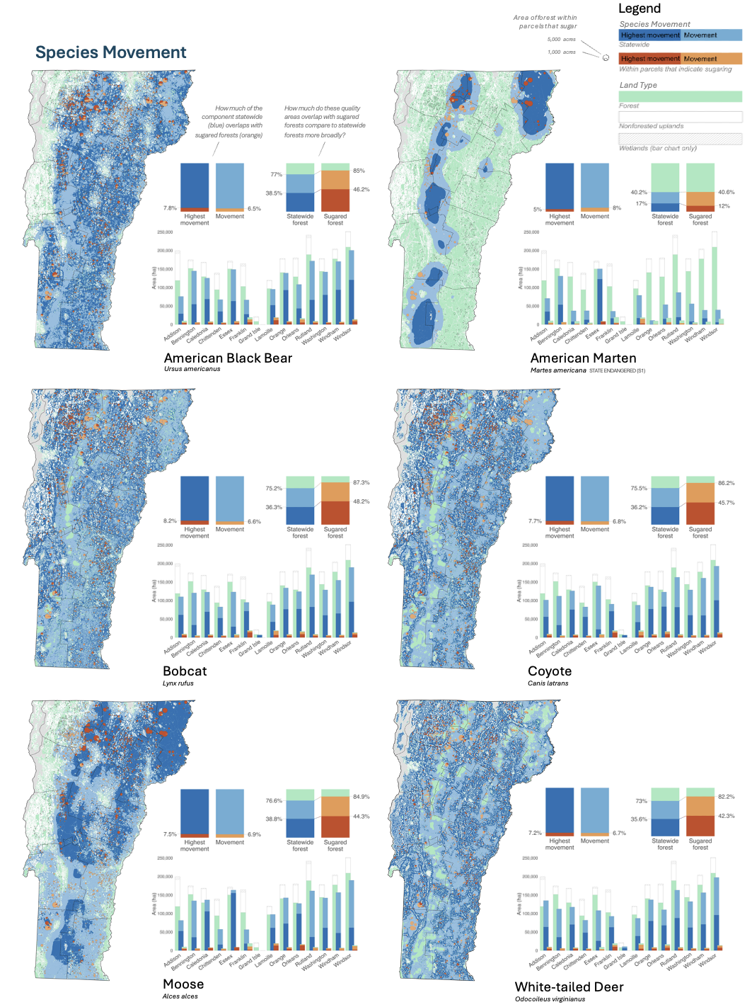
For my graduate thesis with the UVM Field Naturalist Program, I partnered with the FPR Forest Legacy Program to explore the relationship between sugaring and wildlife. Beyond geospatially identifying and characterizing forests where sugaring occurs, I also had the pleasure of surveying 20 sugarbushes across the state to understand vegetation structure and diversity, as well as which birds and mammals are found at the center and along the edge of each sugarbush.
It turns out flying squirrels are very common! And mice frequently scurry across the tubes. While most species did not appear to be impacted by the tubing, more research is needed to determine impact of tubing on moose.
Forest Ecosystem Monitoring Cooperative
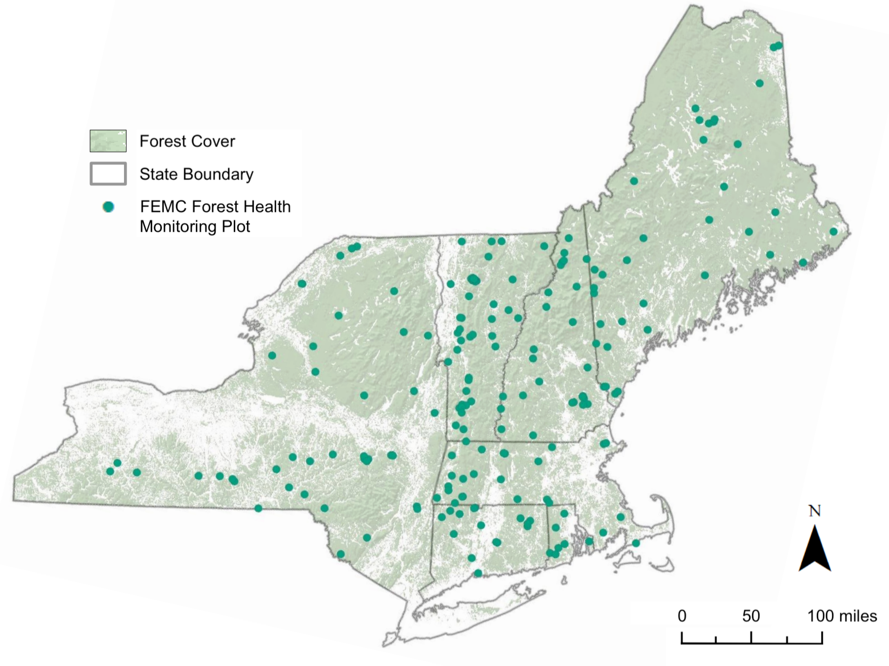
Over 5 years with FEMC has been an wonderful way to get to know the ‘who’s who’ of the natural resources community across the Northeast, from agency personnel at USDA Forest Service and state-level organizations, consultants, folks working with non-profit, and everyone in between. Working with FEMC has meant moving many projects across the finish line at once, learning new skills with each. It has allowed me to keep up with the science and meet amazing people along the way.
Here, I’ve highlighted several projects that showcase the many hats I’ve worn throughout my time with FEMC.
Southwestern Kansas
While leading field crews monitoring nest success of Lesser Prairie-chickens, I also developed and conducted a survey to see if the recent wildlife had influenced colonization of invasive saltcedar. Surveys showed most trees were top-killed but resprouted vigorously from their roots. A year and a half after the fire, these sprouts were already over 2 meters tall! As prairie-chicken are sensitive to tall features on the landscape (being the prey of many birds of prey that perch on these features), these findings suggest that wildlife is insufficient in keeping tall features from the landscape.
I published my research in Priarie Naturalist (2022).